Chapter 6: Geometric Transformation and Eigen Decomposition. In the chapter mind map this icon labels Projection. The discussion below is excerpted and lightly edited from § Projection in Mathematics for AI and Machine Learning.

An orthogonal projection is a special type of linear transformation that maps a vector onto its "closest point" in a subspace. Unlike the transformations discussed above, it is not a bijection (not invertible) because it collapses information, mapping multiple vectors to the same point.

While we focus on orthogonal projection (where the projection direction is perpendicular to the subspace), there also exist oblique projections. In an oblique projection, vectors are still collapsed onto a subspace, but the "shadow" is cast at an angle. Both types are singular and non-invertible, but orthogonal projection is far more common in AI/ML because it minimizes the "distance" (error) between the original vector and its projection.

In 2D, a projection matrix projects vectors onto a subspace (like a line). This generalizes the vector-to-vector projection discussed in Section the referenced section of the matrix chapter to matrix-based projections onto subspaces.

Projection onto a line through the origin with unit direction vector $\mathbf{u}$:

This is a special case of the general projection matrix $P = X(X^\top X)^{-1}X^\top$ discussed in detail in Property the referenced section. When projecting onto a single unit vector $\mathbf{u}$, the term $(X^\top X)^{-1}$ becomes $(\mathbf{u}^\top \mathbf{u})^{-1} = 1$, simplifying the expression to an outer product.

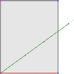
As shown in the book figure a 2D projection transformation collapses the object onto a lower-dimensional space (e.g., projecting 2D points onto a 1D line). Projection onto the $x$-axis (red dashed line) flattens the square into a line segment on the $x$-axis, while projection onto an arbitrary line (green dash-dot line) flattens it onto that line. The vertices and their corresponding projection points are highlighted; connecting any vertex to its projection yields the residual vector $\mathbf{R}$, which is always orthogonal to the subspace of projection.