Reparameterization Trick
Chapter 16: Variational Inference and Latent Variables — Reparameterization Trick
From the book
Chapter 16: Variational Inference and Latent Variables. In the chapter mind map this icon labels Reparameterization Trick. The discussion below is excerpted and lightly edited from § Reparameterization Trick in Mathematics for AI and Machine Learning.
The ELBO contains an expectation over $q_{\boldsymbol\phi}(\mathbf z | \mathbf x)$, which depends on $\boldsymbol\phi$. To enable gradient-based optimization, we use the reparameterization trick:
Instead of sampling $\mathbf z \sim q_{\boldsymbol\phi}(\mathbf z | \mathbf x) = \mathcal{N}(\boldsymbol\mu_{\boldsymbol\phi}(\mathbf x), \mathrm{diag}(\boldsymbol\sigma_{\boldsymbol\phi}^2(\mathbf x)))$, we:
1. Sample $\boldsymbol\epsilon \sim \mathcal{N}(\mathbf 0, \mathbf I)$ (independent of $\boldsymbol\phi$) 2. Compute $\mathbf z = \boldsymbol\mu_{\boldsymbol\phi}(\mathbf x) + \boldsymbol\sigma_{\boldsymbol\phi}(\mathbf x) \odot \boldsymbol\epsilon$ (element-wise multiplication)
This reparameterization makes $\mathbf z$ a differentiable function of $\boldsymbol\phi$ (through $\boldsymbol\mu_{\boldsymbol\phi}$ and $\boldsymbol\sigma_{\boldsymbol\phi}$), enabling backpropagation. With reparameterization, the ELBO becomes:
The reparameterization trick enables gradient-based optimization of the ELBO by making the sampling operation differentiable.
the book figure visualizes the reparameterization trick transformation. The left panel shows samples from the base noise distribution $\boldsymbol\epsilon \sim \mathcal{N}(\mathbf{0}, \mathbf{I})$ (gray points), which is independent of the encoder parameters $\boldsymbol\phi$. The red star marks the mean of this distribution at the origin $(0, 0)$. The right panel shows the transformed latent codes $\mathbf{z} = \boldsymbol\mu_{\boldsymbol\phi}(\mathbf{x}) + \boldsymbol\sigma_{\boldsymbol\phi}(\mathbf{x}) \odot \boldsymbol\epsilon$ (purple points), which are shifted by the mean $\boldsymbol\mu$ and scaled by the standard deviation $\boldsymbol\sigma$. The red stars mark the origin $(0, 0)$ and the transformed mean $\boldsymbol\mu$, and the black arrow indicates the mean shift from the origin to $\boldsymbol\mu$. This visualization makes concrete how the reparameterization trick isolates stochasticity in the noise variable $\boldsymbol\epsilon$, making the latent code $\mathbf{z}$ a deterministic, differentiable function of the encoder parameters. This enables gradient-based optimization because gradients can flow through the deterministic transformation, whereas direct sampling from $q_{\boldsymbol\phi}(\mathbf{z}|\mathbf{x})$ would block gradient flow.
What this drawing shows
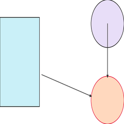
What you see. Boxes for $\mu,\sigma$ and $\epsilon$ fixed; arrows to sampled $z$ grow, illustrating $z = \mu + \sigma \odot \epsilon$.
In the mind map. Chapter 16 — Reparameterization Trick. See From the book above for definitions, figures, and worked examples.
Where to read next
Read the full definitions, figures, and worked examples in Chapter 16: Variational Inference and Latent Variables — see the mind-map node Reparameterization Trick.