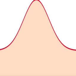
Gaussian Distribution
Chapter 13: Probability and Random Variables — Gaussian,Uniform,Bernoulli
From the book
Chapter 13: Probability and Random Variables. In the chapter mind map this icon labels Gaussian,Uniform,Bernoulli. The discussion below is excerpted and lightly edited from § Example: Gaussian Mixture Model in Mathematics for AI and Machine Learning.
Here we use the Gaussian (normal) distribution, denoted as $\mathcal{N}(\mu, \sigma^2)$, which represents a continuous distribution with mean $\mu$ and variance $\sigma^2$. For $\mathcal{N}(\mu, 1)$ (variance 1), the probability density function is $\phi(x-\mu) = \frac{1}{\sqrt{2\pi}} \exp\left(-\frac{(x-\mu)^2}{2}\right)$, where $\phi(z) = \frac{1}{\sqrt{2\pi}} e^{-z^2/2}$ is the standard normal density. (A formal definition of the Gaussian distribution is given in the "Gaussian Distribution" section later.)
Let $X\in\{0,1\}$, $Y\sim\mathcal N(X,1)$, and $P(X=1)=q$. Compute $p(1\mid y)$.
What this drawing shows
What you see. Represents the normal distribution and its mean/covariance geometry.
In the mind map. Chapter 13 — Gaussian,Uniform,Bernoulli. See From the book above for definitions, figures, and worked examples.
Where to read next
Read the full definitions, figures, and worked examples in Chapter 13: Probability and Random Variables — see the mind-map node Gaussian,Uniform,Bernoulli.