Langevin Equation
Chapter 18: Langevin Dynamics and Sampling — Langevin Equation
From the book
Chapter 18: Langevin Dynamics and Sampling. In the chapter mind map this icon labels Langevin Equation. The discussion below is excerpted and lightly edited from § Langevin Equation in Mathematics for AI and Machine Learning.
To illustrate how Langevin dynamics works, consider sampling from a 1D Gaussian distribution $p(x) = \mathcal{N}(x; \mu, \sigma^2)$ with $\mu = 0$ and $\sigma^2 = 1$.
Using the discrete-time update rule with step size $\eta = 0.01$:
Starting from $x_0 = 5$ (far from the mean), after 40,000 iterations:
- The sample distribution converges to $\mathcal{N}(0, 1)$
- The trajectory shows the particle moving toward the mean while being perturbed by noise
- The algorithm successfully explores the entire distribution
the book figure demonstrates the convergence of Langevin dynamics to the $\mathcal{N}(0, 1)$ distribution. Starting from $x_0 = 5$ (far from the mean), the top panel shows the trajectory converging toward $\mu = 0$ with noise perturbations, with the starting point marked by a green dot. The bottom panel compares the high-resolution histogram of samples (all steps, 150 bins) with the true $\mathcal{N}(0, 1)$ distribution, confirming successful convergence.
What this drawing shows
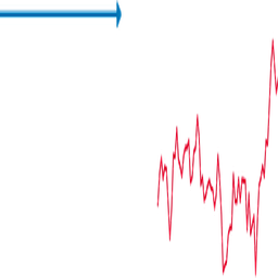
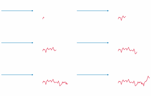
What you see. Blue drift $\nabla\log p\,dt$ arrow fixed; red Wiener path $dW_t$ grows along the time axis in the SDE $dx_t = \nabla\log p\,dt + \sqrt{2}\,dW_t$.
In the mind map. Chapter 18 — Langevin Equation. See From the book above for definitions, figures, and worked examples.
Where to read next
Read the full definitions, figures, and worked examples in Chapter 18: Langevin Dynamics and Sampling — see the mind-map node Langevin Equation.