SDE Sample Path
Chapter 18: Langevin Dynamics and Sampling — Diffusion Preview
From the book
Chapter 18: Langevin Dynamics and Sampling. In the chapter mind map this icon labels Diffusion Preview: Continuous-Time SDEs. The discussion below is excerpted and lightly edited from § Preview: Continuous-Time Limits in Mathematics for AI and Machine Learning.
The discrete Langevin dynamics algorithm studied is a time-discretized version of a continuous stochastic process. In the subsequent chapters, we will formalize this connection by introducing stochastic differential equations (SDEs).
Chapter the referenced section will show how the discrete update converges to a continuous SDE as the step size $\eta \to 0$. This continuous-time perspective provides deeper theoretical understanding and enables the development of more sophisticated sampling algorithms.
Chapter the referenced section will reveal that the same probability distribution can be generated by both stochastic (SDE) and deterministic (ODE) processes, leading to the concept of probability flow ODEs that enable fast deterministic sampling.
Finally, Chapter the referenced section will describe how probability distributions evolve over time through the Fokker-Planck equation, providing the highest-level mathematical description of diffusion processes.
the book figure provides a preview of the Fokker-Planck perspective by tracking the evolution of a cloud of 2000 particles under Langevin dynamics for a 2D mixture of Gaussians. Instead of following a single trajectory, this visualization shows how the density of particles evolves over time. At $t=0$, particles start in a tight cluster far from the data distribution (low-probability region). At $t=30$, the deterministic drift dominates: the score field acts like a strong wind, pushing the cloud rapidly toward the high-density regions. Notice how the cloud stretches—this stretching is exactly what the advection term in the Fokker-Planck equation describes. At $t=1000$, the system reaches equilibrium: the particles have arrived at the modes, but crucially, they don't collapse to single points. The diffusion term (random noise) keeps them spreading out, exactly filling the volume of the theoretical distribution. This visualization demonstrates that Langevin dynamics on individual samples is equivalent to Fokker-Planck evolution on probability densities, providing a bridge between the particle-level and distribution-level perspectives.
Together, these chapters demonstrate that Langevin dynamics is not merely a heuristic algorithm, but a principled application of stochastic calculus to sampling from probability distributions. The noise in Langevin dynamics is not a computational artifact—it is the mathematical mechanism that ensures correct sampling from the target distribution.
What this drawing shows
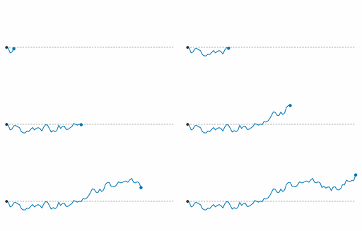
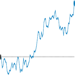
What you see. Brownian sample path fluctuates around dashed $\mathbb{E}[x_t]=0$; animation grows the noisy trajectory from $t{=}0$ to $T$.
In the mind map. Chapter 18 — Diffusion Preview: Continuous-Time SDEs. See From the book above for definitions, figures, and worked examples.
Where to read next
Read the full definitions, figures, and worked examples in Chapter 18: Langevin Dynamics and Sampling — see the mind-map node Diffusion Preview: Continuous-Time SDEs.