Diffusion Model
Chapter 21: Fokker-Planck and Distribution Dynamics — Diffusion Models and Generative Applications
From the book
Chapter 21: Fokker-Planck and Distribution Dynamics. In the chapter mind map this icon labels Apps: Diffusion Model. The discussion below is excerpted and lightly edited from § Diffusion Models and Generative Applications in Mathematics for AI and Machine Learning.
In diffusion models, the forward process is designed to gradually add noise to data. For a pure diffusion process without drift (corresponding to the Variance Exploding formulation):
where $\beta(t) > 0$ is a noise schedule that controls the diffusion rate over time.
This is the heat equation (also called the diffusion equation), which describes pure diffusion without drift.
the book figure visualizes the forward diffusion process in diffusion models, demonstrating how the heat equation destroys information over time. The top panel shows the initial distribution at $t=0$: a complex, multimodal structure with three distinct peaks representing structured data with high information content. The middle panel shows the distribution at $t=1.5$: the peaks begin to merge and blur as fine details are lost, entropy increases, and information is destroyed. The bottom panel shows the distribution at $t=15$: convergence to a single, broad, featureless Gaussian (pure noise) with zero information. The dashed line shows the theoretical single Gaussian approximation. This visualization makes concrete the fundamental property of diffusion: it acts as a smoothing operator, and complex data structures are inevitably smoothed into trivial noise—this is the Central Limit Theorem in action. For diffusion models, this forward process transforms any data distribution into pure noise, which can then be reversed using the learned score function.
What this drawing shows
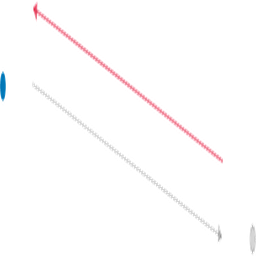
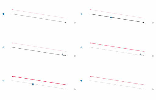
What you see. Blue data (left) and gray noise (right) are fixed anchors; a particle diffuses forward along the black arrow then generates back along the red score-driven arrow, illustrating the train-forward / sample-reverse loop of diffusion models.
In the mind map. Chapter 21 — Apps: Diffusion Model. See From the book above for definitions, figures, and worked examples.
Where to read next
Read the full definitions, figures, and worked examples in Chapter 21: Fokker-Planck and Distribution Dynamics — see the mind-map node Apps: Diffusion Model.