Diffusion Unify
From the book
Chapter 21: Fokker-Planck and Distribution Dynamics. In the chapter mind map this icon labels Unification: Probability Flow ODE. The discussion below is excerpted and lightly edited from § Probability Flow ODE and SDE Unification in Mathematics for AI and Machine Learning. Related material also appears in Chapter 19 (Diffusion Unification: Reverse-Time SDE & ODE Limits), Chapter 20 (ODE-SDE: Probability Flow ODE).
induces a continuity equation (the matrix chapter, equation @eq:continuity-equation):
where $\mathbf{v} = \mathbf{f} - \frac{1}{2}\mathbf{D}\nabla \log p_t$ is the velocity field.
Expanding the divergence and using $\nabla \log p_t = \frac{\nabla p_t}{p_t}$, this becomes:
For state-independent diffusion $\mathbf{D}(t)$, this simplifies to the same Fokker–Planck equation as the SDE.
What this drawing shows
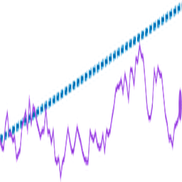
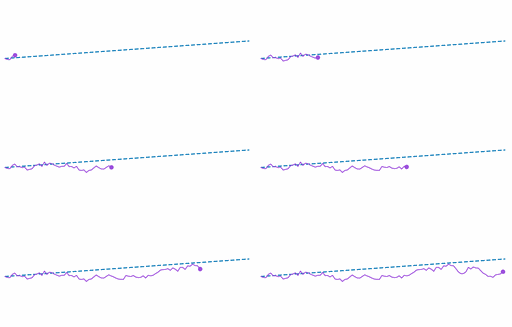
What you see. Blue dashed probability-flow ODE (deterministic drift) fixed; purple SDE sample path grows in time as BM noise around the same flow.
In the mind map. Chapter 21 — Unification: Probability Flow ODE. See From the book above for definitions, figures, and worked examples.
Also appears in Ch. 19 (Diffusion Unification: Reverse-Time SDE & ODE Limits); Ch. 20 (ODE-SDE: Probability Flow ODE).
Where to read next
Read the full definitions, figures, and worked examples in Chapter 21: Fokker-Planck and Distribution Dynamics — see the mind-map node Unification: Probability Flow ODE.
This concept is also referenced in Chapter 19 (Diffusion Unification: Reverse-Time SDE & ODE Limits); Chapter 20 (ODE-SDE: Probability Flow ODE).