Chapter 17: Score Function and Energy-Based Models — Motivation: From Density to Geometry; Score vs Density (also appears in Ch. 18). The passage below is adapted from the manuscript discussion of Score Field. Look in § Motivation: From Density to Geometry; Score vs Density and the surrounding mind-map node "Score vs Density: Visualizing Vector Fields" when reading the print/PDF edition.

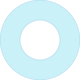
Figure local-information in Chapter 17 contrasts samples from an unknown mixture with the score field ∇_x log p(x) for the same distribution. Observations give local information near data points, but the normalization constant Z remains inaccessible. The score field, drawn as vectors over the density, encodes how log-probability changes locally at every location—and this gradient does not depend on Z. Geometrically, the score points toward higher density, its magnitude measures steepness, and zeros mark extrema. For a bivariate Gaussian the field is radial toward the mean; for a mixture it becomes a weighted blend of component score fields, producing multiple attractors near each mode. Section Score vs Density lists why this vector field is attractive for high-dimensional modeling: it is normalization-free, local, geometric, and directly usable for sampling via Langevin dynamics (developed further in Chapter 18).