Score Function
Chapter 17: Score Function and Energy-Based Models — Score Function
From the book
Chapter 17: Score Function and Energy-Based Models — Score Function. The passage below is adapted from the manuscript discussion of Score Function. Look in § Score Function and the surrounding mind-map node "Score Function: s(x) = ∇_x log p(x)" when reading the print/PDF edition.
Chapter 17 defines the score function as s(x) = ∇_x log p(x), a vector field over data space that points in the direction of increasing probability density. Large magnitude means a steep landscape; zero score marks local extrema such as modes or saddle points. For a Gaussian, the score is s(x) = −Σ⁻¹(x − μ), a radial field pointing toward the mean. The chapter emphasizes that this object is normalization-free: because ∇_x log Z = 0 for any partition constant Z, the score can be computed from an unnormalized density without ever evaluating Z. That property is what makes score-based modeling practical when only local information is available, and it motivates the shift from modeling p(x) directly to modeling its gradient field.
What this drawing shows
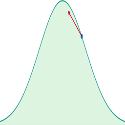
What you see. Shows $s(x)=\nabla\log p(x)$ as a red arrow at a sample point sliding along fixed density $p(x)$ toward the mode; arrow length tracks score magnitude.
In the mind map. Chapter 17 — Score Function: s(x) = ∇_x log p(x). See From the book above for definitions, figures, and worked examples.
Where to read next
Read the full definitions, figures, and worked examples in Chapter 17: Score Function and Energy-Based Models — see the mind-map node Score Function: s(x) = ∇_x log p(x).